Categories
Data Graphics Mashups OpenLayers

The Political Colour of Great Britain

Following on my UK General Elections 2010 Swings map, where circles represent each constituency, with the sizes and colour describing the metrics, I have used a technique that James has been studying, to combine the vote proportions together to produce a single coloured dot for each constituency. The more blue the dot, the higher the proportion of the vote was Conservative. Similarly, red for Labour and Green for the Lib Dems and the other parties and independents.

A purple constituency represents a Labour/Conservative marginal, as blue+red = purple. There are many of these in the Midlands. Similarly, orange areas indicate likely Labour/Lib Dem (or SNP/PC etc) marginals, such as in South Wales, and turquoise areas indicate Conservative/Lib Dem (& other) margins, there are many of these in SW England. Grey dots show three-way marginals, e.g. Hampstead in London.

Because I am using just three colours, to represent three political groupings, the visualisation does not show the variation in results between the Liberal Democrats and the nationalist parties – the SNP and PC in Scotland and Wales respectively.

Some interesting patterns are revealed – the ring of blue/purple around the red/orange centres of London and Birmingham – with no such corresponding ring around Manchester or Newcastle. Scotland’s lack of blue. The straightforward Labour/Conservative split in NW England. East London isn’t quite as safe-Labour as you might think – with the exception of East Ham standing out in bright red.

The benefit of this visualisation is that every vote is included in it – on a regular election map, if one party just fails to win, then an election map won’t show them at all on it. Here, every vote influences the colour of the map. Each circle represents roughly the same number of people – the populations of constituencies are fairly even, with some notable exceptions such as the Isle of Wight (very populated) and the Scottish Islands (very few people.)

You can see the colour map by going to the election visualisation and choosing “Constituency Colour” from the “Other graphs” drop-down. James has produced a regular choropleth map version, which shows the green (SNP/LD) of northern Scotland and blue (Conservative) of southern England strikingly well.

Categories
Data Graphics Mashups

General Election Swings Visualisation

I’ve created a visualisation of the results from the UK general election this month. By default, it shows the most significant swings between parties, for each constituency. By using the options on the right, you can change it to show simple vote counts, overall results, or swings between any two significant parties. I’m using a circle to represent each constituency. The area of the circle is directly proportional to the metric being shown (number of votes, or percentage point swing) with a dynamic key on the right to help out. Click on a circle to see the vote results.

Some Notes:

By choosing “Winning Party” from the “Other” drop down, you see the simplest map – each circle is the same size, and it simply shows the winning results – with the previous winner shown as the colour on the edge of the circle. I think this kind of view is a “best of both worlds” approach – as long as the circles don’t overlap, it has the “fairness” of cartograms (aka “proportional” maps in the BBC’s coverage) while retaining the geographical familiarity of the choropleth (“normal”) map of the UK.

Only Great Britain is included, not Northern Ireland, as the OS Open Data release, which provides the parliamentary boundaries from which the centroids were calculated for the circle locations, does not at the moment include Northern Ireland.

The definition of swing is tricky – swing can only be described as being from one party to another. Choosing which two parties to use for the “headline” swing was tricky. In the end, I’ve chosen to show the swing between the losing and winning party where the seat changed hands, and where it didn’t, the swing between the two parties with the highest number of votes. This means “interesting” swings like in Bethnal Green & Bow are still included. It does however mean that the largest swing is not necessarily shown.

There were a large number of parties contesting seats – in the end I’ve only included parties that got at least 30,000 votes in total, to prevent the lists becoming too long. I’ve also excluded swings where either party in the swing had less than 5% of the vote (i.e. losing their deposit) as such a swing is probably not very meaningful.

In general, a swing between a “small” party and a “large” party is not meaningful anyway, because any voting changes that a large party suffers/gains from are probably to/from another large party, rather than to/from the small party. So, bear this in mind when viewing the swings between (for example) Labour and UKIP. UKIP appears to have gained almost everywhere but actually it was probably another “large” party (Conservatives or Liberal Democrats) that actually got the floating votes.

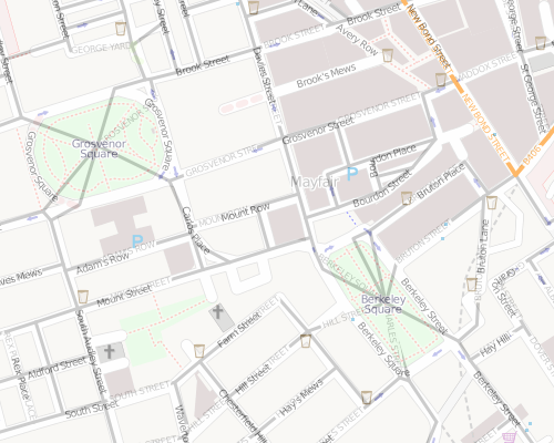
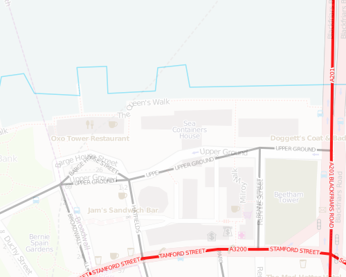
The background imagery was custom-rendered to show the constituency boundaries and be entirely grey – so that the only colours are those representing the party results. Because the boundaries generally run to the low-water mark and estuary mid-lines, whereas OpenStreetMap boundaries generally run to the high-water mark and consider estuaries to be sea rather than river, there are some odd looking estuarine areas (e.g. the Bristol Channel and the Thames Estuary.)

Said another way, this is because of a mismatch between where OpenStreetMap and the parliamentary boundaries commission consider the rivers to stop and the coast to start. I have manually edited two boundaries – NW Bristol sticks far out into the Bristol Channel, and the Medway boundaries also stick far out. NW Bristol’s centroid was also manually moved. There are other, lesser quirks with the data, and being OSM data, not every village is on there yet. I consider the background imagery overall to be “good enough” for the visualisation at hand.

No fancy AJAX was used – the data (about 120KB) is simply loaded into the browser at the start – the visualisation being done entirely on your browser using the OpenLayers API.

It’s not very easy to draw circles in Javascript, so I’ve let OpenLayers do it for me. The two circles that make up the key are actually miniature OpenLayers maps themselves, with a single point feature at the origin of the map. They update in sync with the main map.

The visualisation was ready to go last week but the way Internet Explorer draws the vector graphics (using VML rather than SVG) was causing considerable performance problems, when trying to show all 650-odd constituencies at once. As a work around, the map starts by being zoomed in if you visit the site in IE. Zoom out at your peril!

If you spot any bugs (apart from the IE chronic slowness!) please let me know.

Categories
Data Graphics Mashups OpenLayers OpenStreetMap

Tube Stations in London – Visualisation

I was inspired by seeing this map and associated article on the New York Times website, linked from Going Underground, to create a similar mashup/visualisation of entry/exit volumes from the 300-odd tube stations in London. On their website, Transport for London provide the metrics for entries/exits from the stations, between 2003 and 2008, broken up into rush-hour, regular and weekend travel.

Each circle’s area is directly proportional to the flow numbers for that station (click on the circle to see the numbers.) The circles are rescaled between the first metric (total flows) and the rest, so direct comparison of metrics is possible except between the first and others, Blue circles represent an increase in flow and red a decrease.

If the mass of circles are obscuring each other, zoom in!

You can try it out here.

Some technical notes:

The background map is a custom render of OpenStreetMap data, with the tube lines highlighted in their traditional colour – it doesn’t always look quite “right” when you zoom in, due to the way the lines are tagged in my own copy of the OpenStreetMap database. The stations are even harder to disambiguate, so I’m using a free source from Wikimedia Commons, this means they don’t always line up.

Because your browser gets a copy of all the flow data when you load the page (yes I’ve heard of AJAX) it does run a little slowly in Internet Explorer, particularly the slider bars – these allow you to “drag” through the range of metrics or years.

Categories
Mashups OpenLayers OpenStreetMap

Manchester Map Mashup

I’ve created a mashup of lots of maps of Manchester as a proof-of-concept of how easy it is to mashup using OpenLayers. It’s not particularly pretty but does involve lots of maps.

See it here.

The layers are:

  • OpenStreetMap
  • Ordnance Survey Street View
  • Ordnance Survey 1:25000 First Series (1959)
  • Ordnance Survey New Popular Edition (1948)
  • Marr Map of Housing Conditions (1904)
  • Swire Map of Manchester (1824)

The first four maps are all hosted on OpenStreetMap servers.
The Swire map also contains an inset, dated 1650!

Categories
Mashups OpenLayers OpenStreetMap

Accuracy vs Completeness: OSM vs Meridian 2

[Updated x2] Yesterday’s Ordnance Survey OpenData launch has provided the OpenStreetMap community with a potentially rich set of data to use to complete the map of Great Britain. OpenStreetMap’s accuracy and detail is generally excellent, however a problem which is (very arguably) more important than either accuracy or detail, in a map is that some parts of the country are substantially incomplete.

It’s not that the data quality is poor, it’s that someone with a GPS (or a satellite photo) has never been to that part of the country to gather the data in the first place. There are still significant parts of Scotland and Northern England which have many missing roads. The NPE (out-of-copyright) maps have been useful in starting to fill out these sections, but there’s always going to be a roads missing from a 60-year-old (or older) map.

So, the OS datasets could be very useful. Perhaps the most interesting of the datasets is Meridian 2, it is a vector dataset covering the whole country. One thing that needs to be watched out for though is that Meridian (which is a “complete” dataset of the country) is relatively inaccurate Pixellation or resolution isn’t a problem, it being vector based – but data is quite simplified.

I’ve built a mashup which allows direct comparision of the Meridian and OSM data for Great Britain. I’ve added in most of the available layer files that come with the Meridian package that has been released as part of the OS OpenData initative. The only two areal ones I’ve added are for woodland areas and lakes – everything is linear. I’ve added in labels for the roads and rivers, but no boundaries or point features, at this stage.

You can access the mashup here [now offline] (N.B. Not tested in IE so will probably break horribly in it.) Zooming in reveals the relative coarseness of the Meridian data – although crucially it is “substantially” complete for all but the smallest of roads, for the whole of the UK – not just for the major cities where the OSM contributors mostly live!

Completeness
In the pictures below, the “solid”, thinner roads are Meridian and the fatter roads with “borders” are OSM.

Spot the missing roads in Meridian around Leytonstone in East London [Update 1 – Some sections of motorway are missing from my rendering but are present in the data – it is possible this problem extends to smaller roads too so take these screenshots with a pinch of salt]:

…but go further out of London, and it doesn’t look so good for OSM:

Interestingly, the Park Estate in central Nottingham is missing entirely from Meridian:

The Park Estate is a private estate and the roads are not maintained by the council – this might have something to do with it. I’ll be running around the Park Estate next weekend.

Accuracy
[Update 2 – Meridian is not intended to be used at scales larger than 1:50000, as per its documentation, so I shouldn’t really be comparing it with OSM which generally is based on data recorded at larger scales. So, bear in mind these screenshots are all larger than 1:50000 scale.] It’s difficult to authoritatively judge the relative accuracies of the two datasets without getting out on the streets or looking at aerial imagery – but you can infer a basic measure of accuracy by looking at how roads “wiggle” – or, in the case of the Mayfair squares below, how Meridian converges the square to a point:

Detail
A little unfair to compare the two here, as Meridian 2 was always meant to be a medium-scale dataset, whereas OSM can be all things to all people!

The tiles that make up the imagery are generated on demand (and cached for subsequent use) so may run slowly. You’ll need to zoom in quite a long way before all the features get added to the map. Use the slider on the top left to fade between the OSM and Meridian layers.

The images are derived from Ordnance Survey data © Crown copyright and database right 2010 and OpenStreetMap data which is CC-By-SA OSM and contributors.

Categories
Mashups Technical

OS OpenData is here

It’s the first of April – but it’s not an April Fool – lots of Ordnance Survey medium-scale data has been released today, under a licence compatible with Creative Commons’ Attribution, i.e. you can do what you like with it as long as you attribute and don’t misrepresent the data source.

The best mirror for the data I’ve found is at MySociety – the OS’s own servers have been apparently overloaded since the release went live.

The first use I’ve made of the data is taking the “CodePoint Open” set of postcodes and locations, I’m now using this data as the postcode lookup for OpenOrienteeringMap. If you type in a UK postcode there, it should now take you to exactly the right place. Before, the lookup was using NPEmap data, which was pretty good in general, but someone did spot some glaring errors when they were using it, coincidently, yesterday.

The attribution statement, by the way, can be seen by mousing over the “Jump to Postcode” text.

Categories
Mashups

It’s Back


#uksnow is great – it allows us Brits to indulge in our national pastime of talking about very minor weather events.

Categories
Data Graphics Mashups OpenLayers OpenStreetMap

CensusGIV Prototype Presentation for CASA

My boss (Dr Pablo Mateos) and I gave this presentation today as part of this term’s CASA Seminar series here at UCL. My bit starts at slide 22 (of 60! – we just about managed it in the hour but only by rushing at the end.)

chorogen
CensusGIV – Geographic Information Visualisation of Census Data

View more documents from oliverobrien.

Note that the censusprofiler site mentioned a couple of times in the presentation only has a (very out of date) blog on it at the moment, and the prototype itself is not yet available for general use – with luck, an alpha version will be available to play with by the end of the year.

Categories
Mashups

Visualisation of Census Data

This is the seventh in a series detailing the projects I have worked on at UCL in the last academic year.

My final mashup over the last year is not a “fully working” website, rather an interactive mockup of the sort of web application that I could potentially be building over the next year. It takes some of the data tables from the 2001 UK census, create choropleths of them and shows them on an OpenLayers-powered map. There is the ability to jump to an area by searching on a postcode, and to show, as vector points with name popups, schools. If the site looks similar to some of my other work, that’s because it is – it was cobbled together from existing code, as a “quick” demonstration, rather than being a polished product.

censusprofiler

Categories
Data Graphics Mashups

HEFCE Funding Map

This is the sixth in a series detailing the projects I have worked on at UCL in the last academic year.

hefce

This was a quick mashup to show on a map the latest HEFCE funding round – HEFCE is the government body that decides and awards research funding to the universities around the UK.

This is a vector-based mashup, once again using OpenLayers. For each point, representing a university’s “main” campus, I request a pie-chart from the Google Charts API, and use the resulting image as the marker for the point. There’s no simplification or other generalisation, so, for example, you’ll need to zoom in quite far if you want to make out the different universities in London.

It was cobbled together in about a day, the Thematic Mapping blog was particularly useful for getting the images working as markers.

You can see the mashup here.