Categories
BODMAS OpenLayers

The Great British Bike to Work

Cross-posted from the DataShine blog.

cycle_thumbnail

Here’s a little visualisation created with the DataShine platform. It’s the DataShine Commute map, adapted to show online cycle flows, but all of them at once – so you don’t need to click on a location to see the flow lines. I’ve also added colour to show direction. Flows in both directions will “cancel out” the colour, so you’ll see grey.

London sees a characteristic flow into the centre, while other cities, like Oxford, Cambridge, York and Hull, see flows throughout the city. Other cities are notable for their student flows, typically to campus from the nearby town, such as Lancaster and Norwich. The map doesn’t show intra-zone (i.e. short distance) flows, or ones where there are fewer than 25 cyclists (13 in Scotland as the zone populations are half those in England/Wales) going between each origin/destination zone pair – approximately 0.15% of the combined population.

Visit the Great British Bike to Work Map.

Categories
BODMAS Geodemographics

The Battle of the Roads

ttwm_miltonkeynes

Following on from my two maps of the small-area modal method of travel to work – one map includes cars and so is most interesting for London, and one map excludes cars and so is most interesting for the rest of the country, where cars otherwise dominate – I’ve refined the car-excluding map and introduced a third one.

The Refinement: Map Meaningful Results Only (>10%)

I was mapping the second most popular method of travel to work, after cars. But for many areas, there is no sensible second method. Therefore, I was often mapping results for extremely small numbers of people. One person cycling to work while the other 199 drive, in a small area, does not tell us much. The more interesting result is the lack of a strong non-car travel mode. So, I’ve refined the map to remove the colour where it is representing less than 10% of workers. For areas with good public transport options, or a strong tradition of working from home or walking to work, the map is largely unchanged, but for other areas which are sadly dominated by the motor car, the map now shows large areas of grey.

Four notable areas of greyness are Milton Keynes, the Welsh Valleys, Telford and Middlesbrough. In large conurbations, distinct areas appear, such as Walderslade near Chatham, the outer parts of Swansea or the eastern half of Cannock. London changes little, the nearest car-only area being Sunbury on Thames, which is technically just outside London but within its sphere of influence, if not its public transport options.

Additionally, I previously was also showing a “runner up” non-car mode of travel, where this fell only slightly behind the main mapped mode. This additional mode was shown using vertical stripes. However, I’ve tweaked this so that it is instead always included if, like the primary non-car mode, it also represents at least 10% of workers there. This has most effect in London, where buses are in fact widely used right across London, even if the tube/train mode is also heavily used. So London now is mainly composed purple stripes (bus) on top of orange (tube/train). This change also brings out the cycling mode in a number of other cities, notably Hull and Bristol, cities where public transport is well used – and so was masking the still-popular cycling mode.

The New Map: Road Users Only

I’ve introduced a third map, focusing on road travel only – so I’ve eliminated tube/metro use, as well as working from home.

Do the buses beat the cars (remember though, there are more people on a typical bus than in cars), or do the cyclists beat both? Well – mainly it’s the cars, with most cities and other urban areas showing a walking core, surrounded by cars. Inner city areas often have bus use appearing, typically as a second-place usage (I only show here, unlike above, it where it nearly is as widely used as the main mode) in some sectors, but not others. Leeds and Bradford both show this pattern:

ttwn_leedsbradford

London is the stand-out exception with heavy bus and bike usage, across wide areas well away from the centre. Taxis are also popular with the rich of Kensington.

But in some towns and cities, even the central walkers lose out. Telford is one place with no walking core. Wellingborough/Rushden is another, and Boston. Margate/Ramsgate’s is unusually small. In these places, at least, the car is king of the roads, throughout the urban realm.

Note: Like all the travel to work maps, I’m mapping small-area statistics for the residential location (i.e. home) of people that are of working age. Each small area has a typical working population of around 200 and typically represents two or three average-length residential streets. The maps include non-residential buildings by necessity, as I do not have data to eliminate these, but the colours/stats only represent the nearby residential population, not people who work in these buildings.

ttwm_stamfordhill

Categories
BODMAS Geodemographics

What if There Were No Cars?

Here’s a map of the top method of travel to work, for each “small area” (~250 people) in the UK, for people aged 16-74 and in employment, at the time of the 2011 Census (or try the interactive, zoomable version):

traveltowork_car

The pattern is, fairly evenly, that car use (light blue) dominates except for people living in the very centre of cities, where walking to work (green) is the most popular method. The two big exceptions are London, where rail/metro travel (orange) dominates for the inner city zone, separating the walking core and car-driving outer London ring; and Cambridge, where the cyclists (red) really are king. There are some other interesting results in small areas (e.g. walking is popular in central Leicester but not in the centre of Peterborough), but overall, the map doesn’t tell you much more.

So, I’ve considered what the map would look like if we removed cars from the calculations – what form of transport is used by the people that need to work but don’t own or otherwise have access to cars, either as a driver or passenger? How does the UK commute, without cars, right now – and what might a UK landscape look like without the great rush-hour traffic jam, if the alternatives, pro-rata, were adopted? A whimsical hypothesis – cars are always going to be essential for certain kinds of commutes in certain parts of the UK – but let’s see what happens anyway, as it will still tell us something about public transport provision, city walkability and maybe attitudes to working life in general.

Here is a map of the top carless commute method for small areas, right across Britain:

traveltowork_nocar

(Here is the interactive, zoomable version).

Suddenly, all sorts of interesting trends emerge. In rural areas, working from home dominates – with no public transport, and motorbikes being an uncommon form of transport in the UK, this is the only option. In towns and villages, and in city centres, walking to work dominations. Both are obvious – the interesting results appear if you zoom in:

  • In London, the central walking-to-work area (green) coincides almost perfectly with the congestion charge zone. Other walking areas include the large outer London town centres of Hillingdon, Croydon and Kingston that have been absorbed into the metropolis, and the traditional community of Stamford Hill.
  • Rail/metro (orange) dominates throughout Zones 2-6 London and beyond.
  • London has four major areas of bus dominance (purple) – Burgess Park in the south, Hackney in the north-east, the western Lea Valley in the north and a huge zone surrounding Heathrow Airport in the west. Three of these not surprisingly coincide with areas of poor rail/metro provision, but the western Lea Valley result is interesting – there are two rail lines down through this area with stopping services. However, notably, this area’s most popular employment type is cleaning – cleaners typically have to work nights, where the bus is the only public transport option.
  • York versus Leeds – both have a similarly sized walking core, but then the rest of Leeds has bus users, while York’s outskirts are dominated by cyclists (red). The flatter nature of York is likely the major reason.
  • Buses are pretty crucial in the Birmingham conurbation.
  • Cycling dominates in almost every part of Cambridge but less so in the other famous cycling city, Oxford. In London, Hackney’s famed cycle community actually has roughly equal prominence with both bus and train/metro use.
  • Stoke-on-Trent has a very large walking core, larger than for the larger cities, covering the whole area almost, rather than being surrounded by bus/cycling/train commuters as normally happens. Stoke-on-Trent is actually a conurbation of six towns, with employment scattered throughout rather than concentrated in the normal core. Alternatively this could be due to poor bus provision or a dominance of driving.
  • Ilkley and Bingley like their trains – nearby Keighley and Skipton, nearby and on the same network, don’t. The former two towns perhaps act more as commuter towns for Leeds while the latter two have a tradition of more local employment.
  • The very richest areas have a high proportion of people working at home (brown) – live in help, aka domestic servants? See Knightsbridge and Hampstead Garden Suburb in London, or Sutton Park near Birmingham, are two examples.
  • The new towns in central Scotland seems to have a greater proportion of working-at-home than equivalent new-town areas in England.
  • Fishing communities (yellow – other) are obvious in north-east Scotland:

traveltowork_nocar_fish

These are just a few of the spatial patterns I’ve spotted – there are I’m sure many more interesting ones. Sometimes, removing the dominant factor reveals the interesting map.

The technique of mapping only the most dominant mode of transport has a serious flaw, in that, depending on how you merge or split other transport modes, you can significantly influence which appears “top”. I have merged some modes together (driver+car passenger, train+metro+tram, and taxi+motorbike+other, e.g. boat), hopefully in a meaningful way that shows interesting results without hiding the bigger picture. Another mitigating factor is that, where a second mode of transport has nearly as much use as the first, I include its colour too, in narrow vertical banding, and highlight this in the interactive “area information” panel.

All the maps in this article use the CDRC Maps platform, created by the Consumer Data Research Centre, to map small-area consumer and other demographic data for the UK. Because I am using Census data, I am able to map for the whole of the UK (including Scotland and Northern Ireland), as, for the Census at least, the activity is coordinated across the nations, and while the outputs are arranged differently, they are sufficiently similar to combine and use together with care. The data comes from the National Statistics agencies – the ONS, NRS and NISRA, and is Crown Copyright, licensed under the Open Government Licence.

Have a look at some other CDRC datasets mapped, download the data yourself or find out more about the CDRC.

traveltowork_nocar_cambridge

Categories
BODMAS Conferences

In/Visibility and Difference – Visual Methods Workshop in Berlin

vmw1

I presented a talk on geodemographic mapping, at a visual methods workshop “In/Visibility and Difference” which took place in Berlin at Bard College (formerly the European College of Liberal Arts). The workshop was organised by the TransformIG project at Humboldt University in Berlin, which was also the venue for the keynote part of the meeting. Thank you to the organisers for organising an interesting and intensive workshop which presented a wide variety of visual and geographical techniques which are becoming key ways to structure and analyse sociological studies.

I structured my talk into four sections:

  1. An primer on improving choropleth mapping of socioeconomic data, moving beyond the basic “heat map” by adding regular geographical feaures (see photo below), labels and clipping coverage to populated areas, to explain the demographic patterns and highlight external influences. This is the technique used by DataShine to display Census 2011 aggregate statistics, and CDRC Maps to show geodemographics. I also outlined alternative approaches used by other research groups, such as cartograms and dot density maps.
  2. A tour of the geodemographic maps in CDRC Maps, including the Output Area Classification and a map of the latest Index of Multiple Deprivation. I also touched briefly on the problems of geodemodemographic classifications, where good/poor fits to the classification are typically mapped identically, and the “second choice” classification doesn’t get shown, showing some techniques to try and map these subtleties.
  3. An introduction to more novel methods of mapping demographic data, such as Lives on the Line and Tube Tongues, but highlighting the shortcomings of such maps too.
  4. Finally, a brief mention of mapping more novel datasets, showcasing the Twitter language maps for London and New York – again discussing the flaws as well as strengths of such maps.

vmw_me

I found many of the other talks very interesting – particularly the work by plan b – two performance artists who have essentially tracked their entire outdoor life over the last 8+ years, both creating GPS traces which they have turned into artworks at various scales and on mediums (including a 3D mould), but also temporal activity indicators which they have grouped together into small multiples. They term these the “birch trees” due to their characteristic stripy white/black columns (see top photo). I also liked the striking pictograms created by Migrantas who have created simple and powerful graphics, from stories from the migrant community in Berlin and elsewhere. Their work can be seen on billboards and walls in various places across the city. There was a good talk by Stefan Lindemann on “SuperLUX”, focusing on linear development along commuter lines to Luxembourg City and corresponding population changes – essentially an international take (due to the country’s size) of the more recent “Northern Powerhouse” project to connect the cities of the north of England.

There was one more map “treat” for me at the workshop – the closing keynote given by Caroline Knowles included her investigative journalistic project where she tracked the complete journey of a pair of flip flops – from oil in Kuwait, to factories in South Korea, then to and through the markets in east Africa, to the consumer, and then finally to the rubbish dumps of the region. A map illustrating the life cycle of the flip flops is below.

Thanks to Agata Lisiak and the TransformIG team for inviting me to speak at the workshop and the opportunity to learn as well as disseminate. (Photo credit for the top photo: Agata).

vmw2

Categories
BODMAS

DataShine Wins the BCS Avenza Award for Electronic Mapping

bcsavenza

DataShine Census has won the British Cartography Society’s Avenza Award for Electronic Mapping, for 2015. The glass trophy and certificate were presented to DataShine creator Oliver O’Brien at the award ceremony and gala dinner for the combined BCS/Society of Cartographers conference “Mapping Together” which took place in York, earlier this September. The prize was presented by Peter Jones MBE, the BCS President.

Additionally, DataShine Election was Highly Commended for the Google Award for mapping of the UK General Election 2015.

The book “London: The Information Capital” which DataShine PI James Cheshire co-authored with Oliver Uberti, won three awards at the same ceremony, the Stanfords Award for Printed Mapping, the John C. Bartholomew Award for Thematic Mapping (for Chapter 3 of the book), and the meeting’s grand prize, the BCS Trophy. Dr Cheshire was on hand to receive the trophies and certificates.

The awards cap a successful year for the DataShine project which has seen hundreds of thousands of viewers, several key media articles and four key websites launched, along with a number of variants, most recently including DataShine Scotland Commute which was commissioned by the National Records of Scotland. Full details of the project can be found on the project blog.

neocartography_presentationThe awards were just a small part of a eye-opening and rewarding two-day conference held in central York. A wide variety of talks were held, from academics, company representatives and field enthusiasts. They ranged from detailed discussions of subtle automated cartographical techniques that improve the legendary “Swiss Topo” national maps of Switzerland, to a not-so-serious critique of maps supplied by the floor – a sea/land temperature gradient map proving to be particularly controversial due to its multi-hue, repeating colour ramp. A particular highlight was a discussion on “neocartography” by Steve Chilton, he framed the presentation around an email conversation he’d had with myself and another “experimental” mapper SK53.

The theme “Mapping Together” represented the combination of the annual conferences of the trade-focused BCS with the academic-weighted SOC, the two professional cartography bodies of the UK, for the first time in several years. The format worked well and there was enthusiasm at the meeting for it to be repeated in future years.

bcs_datashinecertificates

This is an extended version of an article that first appeared on the DataShine blog. Photo below courtesy of the Society of Cartographers Publicity Officer.

bcs_avenzaaward2015

Categories
BODMAS Conferences

UKDS Census Applications Conference

census1

I was in Manchester a couple of weeks ago for a UKDS conference on applications of the Census 2011 datasets that have been made available, through the ONS, NOMIS, UKDS and other organisations/projects. The conference was to celebrate the outputs and projects that have happened thus far, now that the Census itself is four years old and most of the main data releases have been made.

It was a good opportunity to present a talk on DataShine, which I made a little more technical than previously, focusing on the cartographical and technological decisions behind the design of the suite of websites.

I enjoyed an interesting talk by Dr Chris Gale, outlining graphically the processes behind creating the 2011 OAC geodemographic classification. Chris’s code, which was open sourced, was recently used by the ONS to create a local-authority level classification. There was also some discussion towards the end of the two-day meeting on the 2021 Census, in particular whether it will happen (it almost certainly well) and what it will be like (similar to 2011 but focused on online responses to cut costs).

All-focus

After the conference close I had time to look around MOSI (the Museum of Science and Industry) which is mainly incorporated around an old railyard, terminus of the world’s oldest passenger railway and containing the world’s oldest station (opened in 1830, closed to passengers in 1844). But I was most impressed by the collection of airplanes in the adjoining hangar (once a lovely old market building), which included a Kamakaze. I also had a quick look around the Whitworth Gallery extension which has been nominated for this year’s Stirling Prize.

census3

Categories
BODMAS Data Graphics London

The City of London Commute

Here’s a graphic I’ve made by taking a number of screenshots of DataShine Commute graphics, showing the different methods of travelling to work in the City of London, that is, the Square Mile area at the heart of London where hundreds of thousands and financial and other employees work.

All the maps are to the same scale and the thickness of the commuting blue lines, which represent the volume of commuters travelling between each home area and the City, are directly comparable across the maps (allowing for the fact that the translucent lines are superimposed on each other in many areas). I have superimposed the outline of the Greater London Authority area, of which the City of London is just a small part at the centre.

ttwf_cityoflondon

There’s lots of interesting patterns. Commuter rail dominates, followed by driving. Car passenger commutes are negligible. The biggest single flow in by train is not from another area of London, but from part of Brentwood in Essex. Taxi flows into the City mainly come from the west of Zone 1 (Mayfair, etc). Cyclists come from all directions, but particularly from the north/north-east. Motorbikes and mopeds, however, mainly come from the south-west (Fulham). The tube flow is from North London mainly, but that’s because that’s where the tubes are. Finally, the bus/coach graphic shows both good use throughout inner-city London (Zones 1-3) but also special commuter coaches that serve the Medway towns in Kent, as well as in Harlow and Oxford. “Other” shows a strong flow from the east – likely commuters getting into work by using the Thames Clipper services from Greenwich and the Isle of Dogs.

Try it out for your own area – click on a dot to see the flows. There is also a Scotland version although only for between local authorities, for now.

Click on the graphic above for a larger version. DataShine is part of the ESRC-funded BODMAS project at UCL. I’ll be talking about this map at the UKDS Census Applications conference tomorrow in Manchester.

Categories
BODMAS OpenLayers Technical

OpenLayers 3 and DataShine

ds_ol3

OpenLayers is a powerful web mapping API that many of my websites use to display full-page “slippy” maps. DataShine: Census has been upgraded to use OpenLayers 3. Previously it was powered by OpenLayers 2, so it doesn’t sound like a major change, but OL3 is a major rewrite and as such it was quite an effort to migrate to it. I’ve run into issues with OL3 before, many of which have since been resolved by the library authors or myself. I was a bit grumbly in that earlier blogpost for which I apologise! Now that I have fought through, the clouds have lifted.

Here are some notes on the upgrade including details on a couple of major new features afforded by the update.

New Features

Drag-and-drop shapes

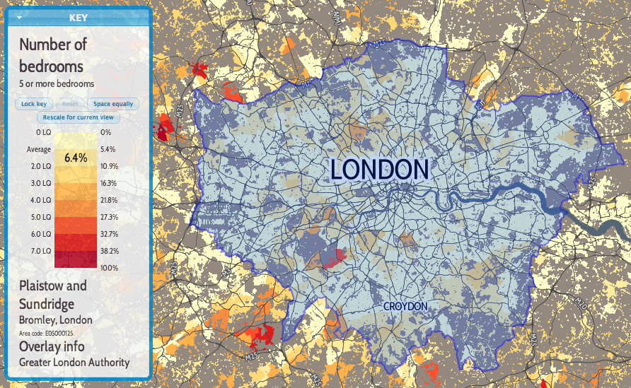
One of the nicest new features of OL3 is drag-and-dropping of KMLs, GeoJSONs and other geo-data files onto the map (simple example). This adds the features pans and zooms the map to the appropriate area. This is likely most useful for showing political/administrative boundaries, allowing for easier visual comparisons. For example, download and drag this file onto DataShine to see the GLA boundary appear. New buttons at the bottom allow for removal or opacity variation of the overlay files. If the added features include a “name” tag this appears on the key on the left, as you “mouse over” them. I modified the simple example to keep track of files added in this way, in an ol.layer.Group, initially empty when added to the map during initialisation.

Nice printing

Another key feature of OL3 that I was keen to make use of is much better looking printing of the map. With the updated library, this required only a few tweaks to CSS. Choosing the “background colours” option when printing is recommended. Printing also hides a couple of the panels you see on the website.

Nice zooming

OL3 also has much smoother zooming, and nicer looking controls. Try moving the slider on the bottom right up and down, to see the smooth zooming effect. The scale control also changes smoothly. Finally, data attributes and credits are now contained in an expandable control on the bottom left.

A bonus update, unrelated to OL3, is that I’ve recreated the placename labels with the same font as the DataShine UI, Cabin Condensed. The previous font I was using was a bit ugly.

Major reworkings to move from OL2 to OL3

UTF Grids

With OpenLayers 3.1, that was released in December 2014, a major missing feature was added back in – support for UTF Grid tiles of metadata. I use this to display the census information about the current area as you “mouse over” it. The new implementation wasn’t quite the same as the old though and I’ve had to do a few tricks to get it working. First of all, the ol.source.TileUTFGrid that your UTF ol.layer.Tile uses expects a TileJSON file. This was a new format that I hadn’t come across before. It also, as far as I can tell, insists on requesting the file with a JSONP callback. The TileJSON file then contains another URL to the UTF Grid file, which OL3 also calls requiring a JSONP callback. I implemented both of these with PHP files that return the appropriate data (with appropriate filetype and compression headers), programmatically building “files” based on various parameters I’m sending though. The display procedure is also a little different, with a new ol.source.TileUTFGrid.forDataAtCoordinateAndResolution function needing to be utilised.

In my map initialisation function:

layerUTFData = new ol.layer.Tile({});

var handleUTFData = function(coordinate)
{
  var viewResolution = olMap.getView().getResolution();
  layerUTFData.getSource().forDataAtCoordinateAndResolution(coordinate, viewResolution, showUTFData);
}

$(olMap.getViewport()).on('mousemove', function(evt) {
  var coordinate = olMap.getEventCoordinate(evt.originalEvent);
  handleUTFData(coordinate);
});

In my layer change function:

layerUTFData.setSource(new ol.source.TileUTFGrid({
  url: "http://datashine.org.uk/utf_tilejsonwrapper.php?json_name=" + jsonName
})

(where jsonName is how I’ve encoded the current census data being shown.)

Elsewhere:

var callback = function(data) { [show the data in the UI] }

In utf_tilejsonwrapper.php:

<?php
header('Content-Type: application/json');
$callback = $_GET['callback'];
$json_name = $_GET['json_name'];
echo $callback . "(";
echo "
{ 'grids' : ['http://datashine.org.uk/utf_tilefilewrapper.php?x={x}&y={y}&z={z}&json_name=$json_name'],
'tilejson' : '2.1.0', 'scheme' : 'xyz', 'tiles' : [''], 'version' : '1.0.0' }";
echo ')';
?>

(tilejson and tiles are the two mandatory parts of a TileJSON file.)

In utf_tilefilewrapper.php:

<?php
header('Content-Type: application/json');
$callback = $_GET['callback'];
$z = $_GET['z'];
$y = $_GET['y'];
$x = $_GET['x'];
$json_name = $_GET['json_name'];
echo $callback . "(";
echo file_get_contents("http://[URL to my UTF files or creator service]/$json_name/$z/$x/$y.json");
echo ')';
?>

Permalinks

The other change that required careful coding to recreate the functionality of OL2, was permalinks. The OL3 developers have stated that they consider permalinks to be the responsibility of the the application (e.g. DataShine) rather than the mapping API, and, to a large extent, I agree. However OL2 created permalinks in a particular way and it would be useful to include OL3 ones in the same format, so that external custom links to DataShine continue to work correctly. To do this, I had to mimic the old “layers”, “zoom”, “lat” and “lon” parameters that OL2’s permalink updated, and again work in my custom “table”, “col” and “ramp” ones.

Various listeners for events need to be added, and functions appended, for when the URL needs to be updated. Note that the “zoom ended” event has changed its name/location – unlike moveend (end of a pan) which sits on your ol.map, the old “zoomend” is now called change:resolution and sets on olMap.getView(). Incidentally, the appropriate mouseover event is in an OL3-created HTML element now – olMap.getViewport() – and is mousemove.

Using the permalink parameters (args):

if (args['layers']) {
  var layers = args['layers'];
  if (layers.substring(1, 2) == "F") {
    layerBuildMask.setVisible(false);
  }
  [etc...]
}
[& similarly for the other args]

On map initialisation:

args = []; //Created this global variable elsewhere.
var hash = window.location.hash;
if (hash.length > 0) {
  var elements = hash.split('&');
  elements[0] = elements[0].substring(1); /* Remove the # */
  for(var i = 0; i < elements.length; i++) {     var pair = elements[i].split('=');     args[pair[0]] = pair[1];   } }

Whenever something happens that means the URL needs an update, call a function that includes this:

var layerString = "B"; //My old "base layer"
layerBuildMask.getVisible() ? layerString += "T" : layerString += "F";
[etc...]
layerString += "T"; //The UTF data layer.
[...]
var centre = ol.proj.transform(olMap.getView().getCenter(), "EPSG:3857", "EPSG:4326");
window.location.hash = "table=" + tableval + "&col=" + colval + "&ramp=" + colourRamp + "&layers=" + layerString + "&zoom=" + olMap.getView().getZoom() + "&lon=" + centre[0].toFixed(4) + "&lat=" + centre[1].toFixed(4);
}

Issues Remaining

There remains a big performance drop-off in panning when using DataShine on mobile phones and other small-screen devices. I have put in a workaround "viewport" meta-tag in the HTML which halves the UI size, and this makes panning work on an iPhone 4/4S, viewed horizontally, but as soon as the display is a bit bigger (e.g. iPhone 5 viewed horizontally) performance drops off a cliff. It's not a gradual thing, but a sudden decrease in update-speed as you pan around, from a few per second, to one every few seconds.

Additional Notes

Openlayers 3 is compatible with Proj4js version 2 only. Using this newer version requires a slightly different syntax when adding special projections. I use Proj4js to handle the Ordnance Survey GB projection (aka ESPG:27700), which is used for the postcode search, as I use a file derived from the Ordnance Survey's Code-Point Open product.

I had no problems with my existing JQuery/JQueryUI-based code, which powers much of the non-map part of the website, when doing the upgrade.

Remember to link in the new ol.css stylesheet, or controls will not display correctly. This was not needed for OL2.

OL3 is getting there. The biggest issue remains the sparsity of documentation available online - so I hope the above notes are helpful in the interim.

ds_ol3overlay2

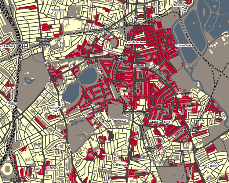
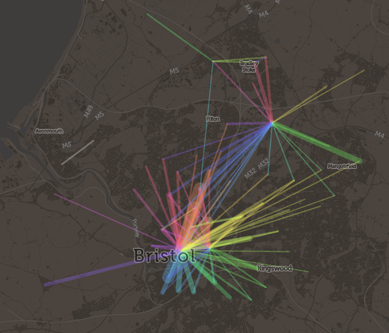
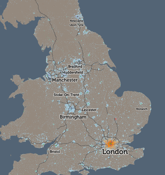
Above: GeoJSON-format datafiles for tube lines and stations (both in blue), added onto a DataShine map of commuters (% by tube) in south London.
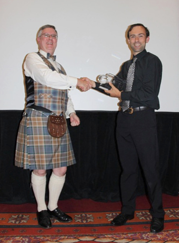
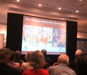
Categories
BODMAS

DataShine: Local Area Rescaling & Data Download

Cross-posted from the Datashine Blog.

DataShine Census has two new features – local area rescaling and data download. The features were launched at the UK Data Service‘s Census Research User Conference, last week at the Royal Statistical Society.

Local Area Rescaling

This helps draw out demographic versions in the current view. You may be in a region where a particular demographic has very low (or high) values compared to the national average, but because the colour breakout is based on the national average, local variation may not be shown clearly. Clicking on the “Rescale for current view” button on the key, will recolour for the current view.

For example, the popularity of London’s underground network with its large population, means that, for other cities with metros or trams, their usage is harder to pick out. So, in Birmingham, the Midland Metro can be hard to spot (interactive version):

metro1

Upon rescaling, just the local results are used when calculating the average and standard deviation, allowing usage variations along the line to be more clearly seen:

metro2

As another example, rescaling can help “smooth” the colours for measures which have a nationally very small count, but locally high numbers – it can remove the “speckle” effect caused by single counts, and help focus on genuinely high values within a small area.

Hebrew speakers in Stamford Hill, north-east London (interactive version):

hebrew1

Upon rescaling, a truer indication of the shape of the core Hebrew-speaking community there can be seen:

hebrew2

Occasionally, the local average/standard deviation values will mean that the colour breakout (or “binning”) adopts a different strategy. This may actually make the local view worse, not better – so click “Reset” to restore the normal colour breakout. Planning/zooming the map will retain the current colour breakout. PDFs created of the current view also include the rescaled colours.

Data Download

On clicking the new “Data” button on the bottom toolbar, you can now download a CSV file containing the census data used in the current view. Like the local area rescaling functionality, this data download includes all output areas (or wards, if zoomed out) in your current view. This file includes geography codes, so can be combined with the relevant geographical shapefiles to recreate views in GIS software such as QGIS.

Next on the DataShine project, we are looking to integrate further datasets – either aggregating certain census ones or including non-census ones such as IMD and IDACI deprivation measures, or pollution.

Categories
BODMAS Geodemographics

DataShine: 2011 OAC

oac2

The 2011 Area Classification for Output Areas, or 2011 OAC, is a geodemographic classification that was developed by Dr Chris Gale during his Ph.D at UCL Geography over the last few years, in close conjunction with the Office for National Statistics, who have endorsed it and adopted it as their official classification and who collected and provided the data behind the classification – namely the 2011 Census.

A geodemographic classification such as this takes the datasets and looks for clusters, where particular places have similar characteristics across many of the variables. It does this on a non-geographic basis, but spatial autocorrelation means that geographic groupings do typically appear – e.g. a particular part of an inner city will typically have more in common with another part of the inner city, than of the suburbs. However, these areas will often also share much in common with other “inner city” parts of cities elsewhere. Names are then assigned, to attempt to succinctly describe the clusters.

As part of the DataShine project, we have taken the classifications, and mapped them, using the DataShine style of restricting the classification colouring to built up areas and (when zoomed in) individual rows of houses. The map is the third DataShine output, following maps of individual census tables and also the new Travel to Work Flows table.

We’re just mapping the eight “Supergroups”, the top-level clusters. A pop-up shows the more detailed groups and subgroups, and you can find pen-portraits for all these classifications on the ONS website.

Click on the box for an individual supergroup, in the key at the top, to see a map showing just that supergroup on its own. For example, here are the “Cosmopolitan” dwellers of London:

oac3

Like 2011 OAC itself, the map covers all of the UK, including Scotland and Northern Ireland. For the latter, there is no Ordnance Survey Open Data which is how we created the building/urban outlines, so we have improvised with data from OpenStreetMap and NISRA (Northern Ireland Statistics).

The map is part of DataShine, an output of the BODMAS project, but also is in conjunction with the the new Consumer Research Data Centre, an ESRC Data Investment which is being set up here at UCL and other institutions. As such, there is a CDRC version of the map.

As part of the BODMAS project we have also been studying the quality of fit of 2011 OAC for different parts of the UK, and techniques to visualise the uncertainty and quality of the classifications. We will be presenting these findings at the Uncertainty workshop at the GIScience conference in Vienna, later this month.

Direct link to the map.
See also the DataShine blog.