Cross-posted to the 360 Here blog.
As a follow-up to my intro post about Tube Heartbeat, here’s some notes on the API usage that allowed me to get the digital cartography right, and build out the interactive visualisation I wanted to.
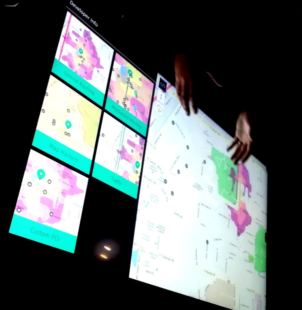
The key technology behind the visualisation is the HERE JavaScript API. This not only displays the background HERE map tiles and provides the “slippy map” panning/zoom and scale controls, but also allows the transportation data to be easily overlaid on top. It’s the first project I’ve created on the HERE platform and the API was easy to get to grips with. The documentation includes plenty of examples, as well the API reference.
The top feature of the API for me is that it is very fast, both on desktop browsers but also on smartphones. I have struggled in the past with needing to optimise code or reduce functionality, to show interactive mapped content on smartphones – not just needing to design a small-screen UI, but dealing with the browser struggling to show sometimes complex and large-volume spatial data. The API has some nice specific features too, here’s some that I used:
Arrows
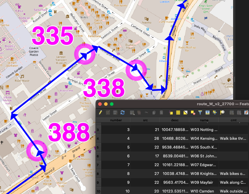
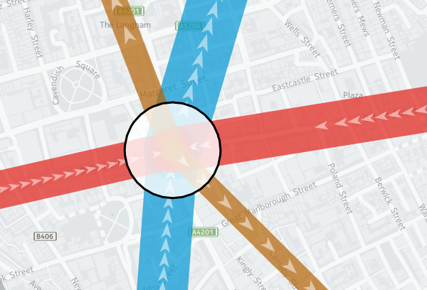
One of the smallest features, but a very nice one I haven’t come across elsewhere, is the addition of arrows along vector lines, showing their direction. Useful for routing, but also useful for showing which flow is currently being shown on a bi-directional dataset – all the lines on Tube Heartbeat use it:
var strip = new H.geo.Strip();
strip.pushPoint({ lat: startLat, lng: startLon });
strip.pushPoint({ lat: endLat, lng: endLon });

var polyline;
var arrowWidth = 0.5; /* example value */

polyline = new H.map.Polyline(
	strip, {
		style: { ... },
		arrows: {
			fillColor: 'rgba(255, 255, 255, 0.5)',
			frequency: 2,
			width: arrowWidth,
			length: arrowWidth*1.5
		}
	}
);

polyline.zorder = lines[lineID].zorder;
The frequency that the arrows occur can be specified, as well as their width and length. I’m using quite elongated ones, which are 3 times as long as they are wide, and occupy the middle half of the arrow (above/below certain flow thresholds, I used different numbers). A frequency of 2 means there is an arrow-sized gap between each one. Using 1 results in a continuous stream of arrows. (N.B. Rendering quirks in some browsers mean that other gaps may appear too.) Here, the blue and red segments have a frequency of 1 and a width of 0.2, while the smaller flows in the brown segments are shown with the frequency of 2 and width of 0.5 in the example code above:
Z-Order
Z-order is important so that the map has a natural hierarchy of data. I decided to use an order where the busiest tube lines were generally at the bottom, with the quieter lines being layered on top of them (i.e. having a higher Z-order). Because the busier tube lines are shown with correspondingly fatter vector lines on the map, the ordering means that generally all the data can be seen at once, rather some lines being hidden. You can see the order in the penultimate column of my lines data file (CSV). I’m specifying z-order simply as a custom object “zorder” on the H.map.Polyline, as shown in the code sample above. This then gets used later when assembling the lines to draw, in a group (see below).
Translucency
I’m using translucency both as a cartographical tool and to ensure that data does not otherwise become invisible. The latter is simply achieved by using RGBA colours rather than the more normal hexadecimals; that is, colours with a opacity specified as well as the colour components. In the code block above, “rgba(255, 255, 255, 0.5)” gives white arrows which are only 50% opaque. The tube lines themselves are shown as 70% opaque – specified in lines data file along with the z-order – this allows their colour to appear strongly while allowing other lines or background map features/captions, such as road or neighborhood names, to still be observable.
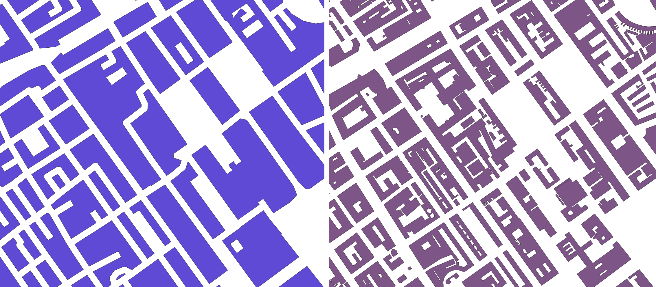
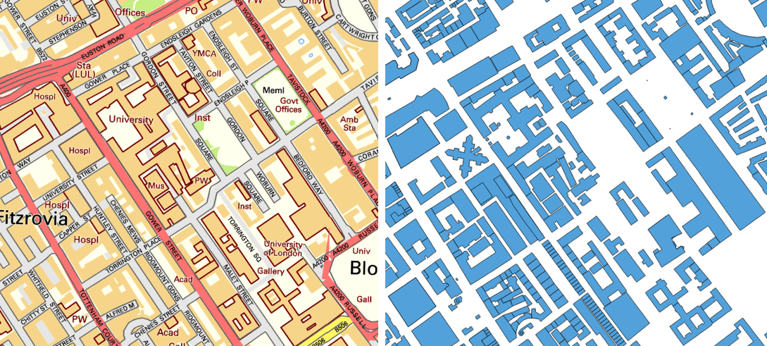
While objects such as the tube lines can be made translucent by manipulating their colour values, layers themselves always display at 100% opacity. This is probably a good thing because translucent map image layers could look a mess, if you layered multiple ones on top of each other, but it means you need to use a different technique if you want to tint or fade a layer. Because even the simplified “base” background map tiles from HERE for London have a lot of detail on them, and the “xbase” extra-simplified ones don’t have enough for my purposes, I needed a half-way house approach. I acheived this by creating a geographical object in code and placing it on top of the layers:
var tintStyle = {
	fillColor: 'rgba(240, 240, 240, 0.35)'
};
var rect = new H.map.Rect(
	new H.geo.Rect(	42, -7, 58, 7 ),
	{ style: tintStyle }
);
map.addObject(rect);
The object here is a very light gray box, at 35% opacity, with an extent that covers all of the London area and well beyond. In HERE JavaScript API, such objects automatically go on top of the layers. My tint doesn’t affect the lines or stations, because I add two groups, containing them, after my rectangle:
var stationGroup = new H.map.Group();
var segGroup = new H.map.Group();
map.addObject(segGroup);
map.addObject(stationGroup);
Object Groups
I can add and remove objects from the above groups rather than directly to the map object, and the groups themselves remain in place, ordered above my tint and the background map layers. Objects are drawn in the order they appear in the group, the so-called “Painters Algorithm“, hence why I sort using my previously specified “zorder” object’s value, earlier:
function segSort(a, b)
{
	var lineA = parseInt(a.zorder);
	var lineB = parseInt(b.zorder);
	if (lineA > lineB) return 1;
	if (lineA < lineB) return -1;
	return 0;
}

var segsToDraw = [];
segGroup.removeAll();

...

segsToDraw.sort(segSort);
for (var i in segsToDraw)
{
	segGroup.addObject(segsToDraw[i]);
}
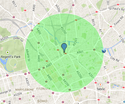
Circles
There are super easy to create and illustrate the second reason that I very much like the HERE JavaScript API. The code is obvious:
var circle = new H.map.Circle(
	{
		lat: Number(stations[i].lat),
		lng: Number(stations[i].lon)
	},
	radius,
	{
		style: {
			strokeColor: stationColour,
			fillColor: 'rgba(255, 255, 255, 0.8)',
			lineWidth: 3
		}
	}
);
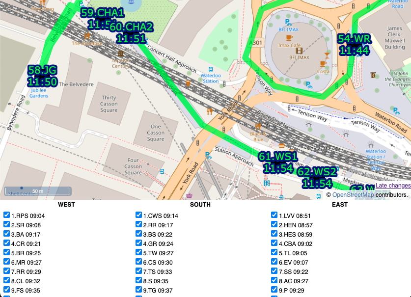
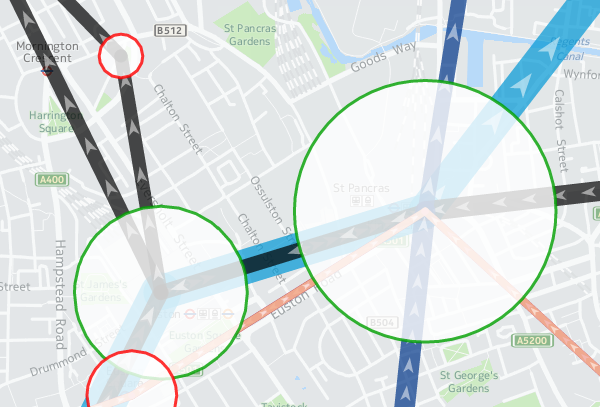
These are my station circles. They are thickly bordered white circles, as is the tradition for stations on maps of the London Underground as well as many other metros worldwide, but with a little bit of translucent to allow background map details to still be glimpsed. Here you can see the circle translucencies, as well as those on the lines, and the arrows themselves, the lines also being ordered as per the z-order specification, so that the popular Victoria line (light blue) doesn't obscure the Northern line (black):
Other Technologies
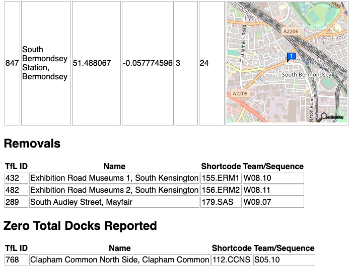
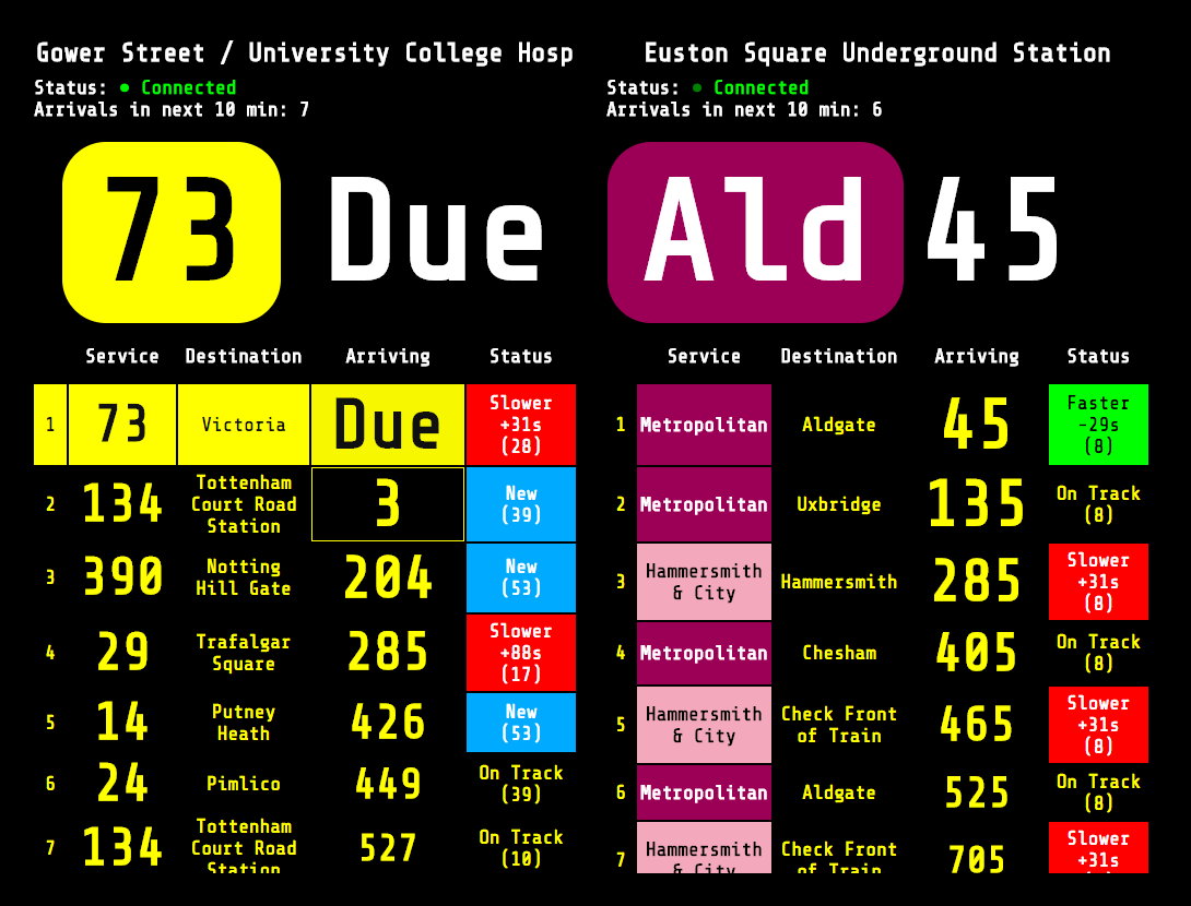
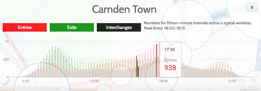
As well as the HERE JavaScript API, I used JQuery to short-cut some of the non-map JavaScript coding, as well as JQueryUI for some of the user controls, and the Google Visualization API (aka Google Charts) for the graphs. Google's Visualization API is full-featured, although a note of caution: I am using their new "Material" look, which works better on mobile and looks nicer too than their regular "Classic" look - but it is still very much in development - it is missing quite a few features of the older version, and sometimes requires the use of configuration converters - so check Google's documentation carefully. However, it produces nicer looking charts of the data, a trade-off that I decided it was worth making:
These are just some of the techniques I used for Tube Heartbeat, and I only scratched at the surface of the HERE APIs, there are all sorts of interesting ones I could additionally incorporate, including some you might not expect, such as a Weather API.
Try out Tube Heartbeat for yourself.
Background map tiles shown here are Copyright HERE 2016.